
Guitar Math
| 02/01/2026 | Written By: Kim Ippolito |
Primer
Note Frequencies
There are twelve notes in the scale
(C,C#,D,D#,E,F,F#,G,G#,A,A#,B), each a semitone
apart, where the relative
frequency (Hz) of each note is calculated by:
Freq(Note) = 2^(1/12) * Freq(Note@semitone below)
This scale is repeated per octave
, such that each octave
is double the frequency of previous octave:
Freq(Note@OctaveN) = 2*Freq(Note@OctaveN-1)
By defining the reference frequency C0 as 16.35 Hz, we can calculate the frequency of any note in any octave. A standard-tuned 24-fret guitar covers the range of E2-E6. The frequencies (in Hz) for each of these notes is shown in both the figure and table below.
![]()
|
Octave |
||||||
|
2 |
3 |
4 |
5 |
6 |
||
|
Note |
C |
65.41 |
130.82 |
261.64 |
523.28 |
1046.56 |
|
C# |
69.299 |
138.6 |
277.2 |
554.4 |
1108.79 |
|
|
D |
73.42 |
146.84 |
293.68 |
587.36 |
1174.72 |
|
|
D# |
77.786 |
155.57 |
311.14 |
622.29 |
1244.58 |
|
|
E |
82.411 |
164.82 |
329.65 |
659.29 |
1318.58 |
|
|
F |
87.312 |
174.62 |
349.25 |
698.49 |
1396.99 |
|
|
F# |
92.504 |
185.01 |
370.01 |
740.03 |
1480.06 |
|
|
G |
98.004 |
196.01 |
392.02 |
784.03 |
1568.07 |
|
|
G# |
103.83 |
207.66 |
415.33 |
830.66 |
1661.31 |
|
|
A |
110.01 |
220.01 |
440.02 |
880.05 |
1760.1 |
|
|
A# |
116.55 |
233.09 |
466.19 |
932.38 |
1864.76 |
|
|
B |
123.48 |
246.96 |
493.91 |
987.82 |
1975.64 |
|
Note that the relationship between adjacent notes is exponential rather than linear - i.e. the notes are not evenly spaced, but grow in distance for each higher note.
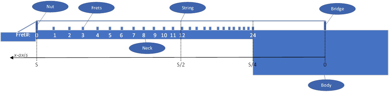
Guitar Fretboard
On a standard-tuned guitar, these notes (and octaves) appear on the fretboard as follows:
|
|
|
Fret# |
||||||||||||||||||||||||
|
0 |
1 |
2 |
3 |
4 |
5 |
6 |
7 |
8 |
9 |
10 |
11 |
12 |
13 |
14 |
15 |
16 |
17 |
18 |
19 |
20 |
21 |
22 |
23 |
24 |
||
|
String # |
1 |
E4 |
F4 |
F#4 |
G4 |
G#4 |
A4 |
A#4 |
B4 |
C5 |
C#5 |
D5 |
D#5 |
E5 |
F5 |
F#5 |
G5 |
G#5 |
A5 |
A#5 |
B5 |
C6 |
C#6 |
D6 |
D#6 |
E6 |
|
2 |
B3 |
C4 |
C#4 |
D4 |
D#4 |
E4 |
F4 |
F#4 |
G4 |
G#4 |
A4 |
A#4 |
B4 |
C5 |
C#5 |
D5 |
D#5 |
E5 |
F5 |
F#5 |
G5 |
G#5 |
A5 |
A#5 |
B5 |
|
|
3 |
G3 |
G#3 |
A3 |
A#3 |
B3 |
C4 |
C#4 |
D4 |
D#4 |
E4 |
F4 |
F#4 |
G4 |
G#4 |
A4 |
A#4 |
B4 |
C5 |
C#5 |
D5 |
D#5 |
E5 |
F5 |
F#5 |
G5 |
|
|
4 |
D3 |
D#3 |
E3 |
F3 |
F#3 |
G3 |
G#3 |
A3 |
A#3 |
B3 |
C4 |
C#4 |
D4 |
D#4 |
E4 |
F4 |
F#4 |
G4 |
G#4 |
A4 |
A#4 |
B4 |
C5 |
C#5 |
D5 |
|
|
5 |
A2 |
A#2 |
B2 |
C3 |
C#3 |
D3 |
D#3 |
E3 |
F3 |
F#3 |
G3 |
G#3 |
A3 |
A#3 |
B3 |
C4 |
C#4 |
D4 |
D#4 |
E4 |
F4 |
F#4 |
G4 |
G#4 |
A4 |
|
|
6 |
E2 |
F2 |
F#2 |
G2 |
G#2 |
A2 |
A#2 |
B2 |
C3 |
C#3 |
D3 |
D#3 |
E3 |
F3 |
F#3 |
G3 |
G#3 |
A3 |
A#3 |
B3 |
C4 |
C#4 |
D4 |
D#4 |
E4 |
|
Where:
- String #1=High E=thinnest string towards floor
- String#6=Low E=thickest string towards ceiling
As you can see, any given octave-note can appear on sequential strings - where E4 is the only octave-note that appears on all 6 strings.
To obtain these notes, tension of each individual strings is
set such that the open tuning (Fret #0) produces the desired frequency output,
fopen. Then, for each consecutive fret to produce a single note (semi-tone)
more than the previous, the fret location (![]() ) of a fret (
) of a fret (![]() ) relative to the bridge is defined
as:
) relative to the bridge is defined
as:
![]()
Where S is the scale of the guitar, such as 25.5 inches.
The fundamental frequency produced for each fret is calculated to be:
![]()
Thus:
|
nFret |
L/S |
freq/fopen |
|
|
0 |
1.000 |
1.000 |
Open |
|
1 |
0.944 |
1.059 |
|
|
2 |
0.891 |
1.122 |
|
|
3 |
0.841 |
1.189 |
|
|
4 |
0.794 |
1.260 |
|
|
5 |
0.749 |
1.335 |
|
|
6 |
0.707 |
1.414 |
|
|
7 |
0.667 |
1.498 |
|
|
8 |
0.630 |
1.587 |
|
|
9 |
0.595 |
1.682 |
|
|
10 |
0.561 |
1.782 |
|
|
11 |
0.530 |
1.888 |
|
|
12 |
0.500 |
2.000 |
1 Octave Up |
|
13 |
0.472 |
2.119 |
|
|
14 |
0.445 |
2.245 |
|
|
15 |
0.420 |
2.378 |
|
|
16 |
0.397 |
2.520 |
|
|
17 |
0.375 |
2.670 |
|
|
18 |
0.354 |
2.828 |
|
|
19 |
0.334 |
2.997 |
|
|
20 |
0.315 |
3.175 |
|
|
21 |
0.297 |
3.364 |
|
|
22 |
0.281 |
3.564 |
|
|
23 |
0.265 |
3.775 |
|
|
24 |
0.250 |
4.000 |
2 Octaves Up |
Visually, these positions are shown below:
Plucking a Single String
Fundamental & Harmonic (overtone) Frequencies
To play a note on the guitar, the musician must depress the string at the desired fret and then pluck the string at a position between the fret and the bridge. As a result, the guitar string vibrates at the desired frequency plus at all harmonics (multiples) of that frequency. (These harmonics are also called overtones.)
The harmonics are linear in relationship (i.e. are evenly
spaced). However, since the notes are not evenly spaced, the harmonics don't
always land on a given note. The harmonics that land on a note are considered
harmonic overtones
, while those that don't are considered inharmonic
overtones
.
For instance, if the G2 notes is played (freq=98.004 Hz) on an ideal (perfectly tuned and intonated) guitar, then the closest note to the harmonics are highlighted below (where most of the harmonics don't fall directly on the highlighted notes):
|
Octave |
||||||
|
2 |
3 |
4 |
5 |
6 |
||
|
Note |
C |
65.41 |
130.82 |
261.64 |
523.28 |
1046.56 |
|
C# |
69.2995 |
138.599 |
277.198 |
554.396 |
1108.79 |
|
|
D |
73.4202 |
146.84 |
293.681 |
587.362 |
1174.72 |
|
|
D# |
77.786 |
155.572 |
311.144 |
622.288 |
1244.58 |
|
|
E |
82.4114 |
164.823 |
329.646 |
659.291 |
1318.58 |
|
|
F |
87.3119 |
174.624 |
349.247 |
698.495 |
1396.99 |
|
|
F# |
92.5037 |
185.007 |
370.015 |
740.03 |
1480.06 |
|
|
G |
98.0043 |
196.009 |
392.017 |
784.034 |
1568.07 |
|
|
G# |
103.832 |
207.664 |
415.328 |
830.655 |
1661.31 |
|
|
A |
110.006 |
220.012 |
440.024 |
880.049 |
1760.1 |
|
|
A# |
116.547 |
233.095 |
466.189 |
932.379 |
1864.76 |
|
|
B |
123.478 |
246.955 |
493.911 |
987.821 |
1975.64 |
|
Thus, when you play a single note on the guitar, you are actually producing many overtones (harmonic and inharmonic) rather than just the fundamental frequency.
Fundamental and Harmonic Amplitudes
Due to the nature of the guitar, for a normally plucked string, the fundamental frequency of the produced sound tends to be stronger than the harmonics. When plucked at the center of the string (halfway between fret and bridge), the initial amplitude of each harmonic can be modeled as 1/k (where k is the harmonic number, with 1 being the fundamental).
Note that this relationship is for the ideal case, where the actual relationship may depend on the guitar quality, the design of the bridge (whether fixed or floating), how the string is plucked, the pick (plectrum) material, and user intervention (such as pinch harmonics).
Also, when recording with a pickup, the pickup measures the velocity of the string at that position rather than position of the string at that location. Thus, the pickup measures an amplitude of 1/k rather than 1/k^2. Both of these models are shown in the following chart.
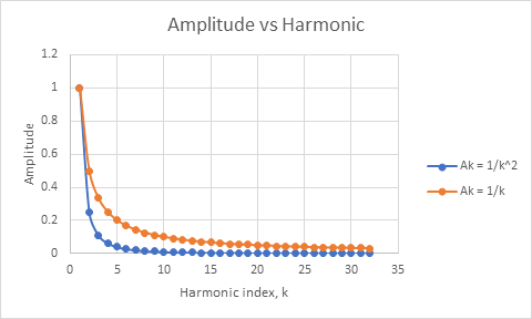
As can be seen, the harmonic intensities drop quickly after the first few harmonics.
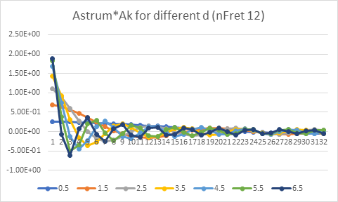
The above plot shows the harmonic amplitudes when the strum location is at the center of the string. However, when strum location, d, is shifted from the center, as is usually the case, the amplitudes are additionally scaled by a sinusoidal.
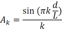
The calculation for ![]() , as observed on the pickup, is:
, as observed on the pickup, is:
The following diagram shows the amplitude factor for different strum locations, d.
Harmonic Damping
The previous plot illustrates the ideal harmonics amplitudes at the start of the pluck. The harmonics decay at a different rate, with the higher frequency harmonics dropping faster than the fundamental. The following plot illustrates the decay over time, per harmonic.
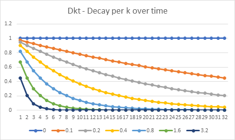
The harmonic damping term ![]() is calculated as:
is calculated as:
![]()
Where ![]() is a constant for the
particular guitar, and
is a constant for the
particular guitar, and ![]() is the time since the
start of the strum.
is the time since the
start of the strum.
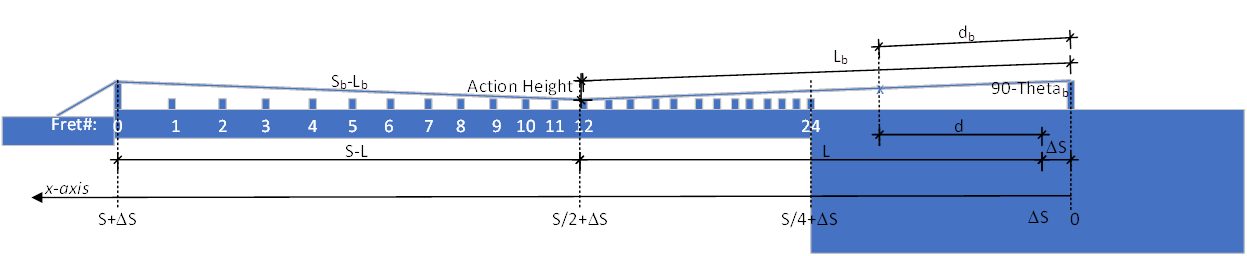
Action Height, Scale Compensation
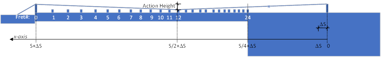
When we press down (clamp) a string at a fret, it is depressed by a distance known
as the action height
. Depressing the string has two affects: (a) the increased
tension increases the frequency, and (b) the increased length decreases the
frequency. The former is more prominent of an effect for steel string
guitars. Thus, all frets, other than fret #0 (open) will have this
intonation
issue. To compensate, the scale length is extended (compensated)
by DS to allow both the fret #0 and
fret #12 to be in tune. All other frets will be slightly off (but much closer
than without compensation). Note that this compensation amount will vary per
string.
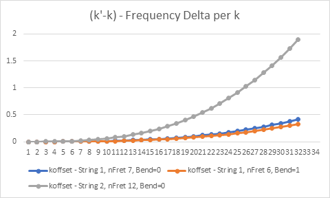
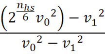
Besides just compensating the fundamental frequency, the harmonics are also impacted, causing the higher frequencies harmonics to be slightly higher than the ideal case. This can be modeled as a modification to the harmonic index, k, such that it becomes an irrational (real) number rather than an integer:
![]()
Where C is a stiffness term.
The amount of string bend also has an impact on the
previously described terms: harmonic amplitude, ![]() , and harmonic damping,
, and harmonic damping, ![]() ; as well as on the standing wave
shape,
; as well as on the standing wave
shape, ![]() , which is described in a following
next section. (The exact formulas are provided in a later section.)
, which is described in a following
next section. (The exact formulas are provided in a later section.)
To retain perfect intonation, the action height per fret, per string, is shown below:
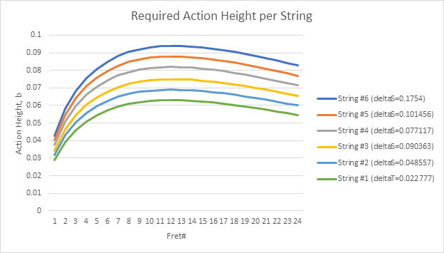
Where the larger compensation (deltaS) values of the thicker strings allow them to have higher action heights compared to the thin strings.
Bending
The previous section introduced the impact of bending the string by the action height. By sliding the string across the fret, this bending value can be further increased. Thus, the model that accounts for the static action height can be used to model the dynamic bending value as well. Thus, the total bend amount (including the action height) can be described by the total distance of the bend, or in terms of the amount of increase to the fundamental frequency, such as in units of half-steps (semitones).
Magnetic Pickup
Pickup Position
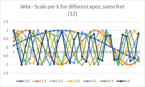
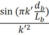
For an acoustic guitar, the sound is produced directly from all frequencies produced by the string vibration, including all harmonics. However, a magnetic pickup only measures velocity of the string at the location of the pickup, xpos. As a result, the measured frequencies are scaled by Wkx, which has the form of a sinusoidal over k, whose shape is a function of the fret depressed and the pickup's x position. Thus, some harmonics (for some frets) may be completely filtered out based upon the pickup location. This filter can be defined as:
![]()
The shape of the ![]() filter, as a function of k, for
fret #12, is shown in the following figure. Each line represents a different
pickup locations.
filter, as a function of k, for
fret #12, is shown in the following figure. Each line represents a different
pickup locations.
To illustrate the Wkx filter for different frets, the following plot shows the plot per fret (0 to 24) given a specific pickup position.
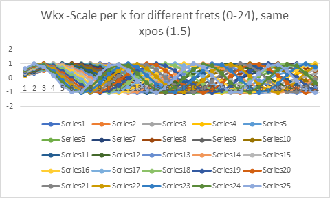
Note that all other previously discussed factors keep the fundamental frequency larger than the harmonics; however, the pickup location can cause the fundamental to be lower than harmonics.
Weighted Sum of all Strings
Up until now, we have been talking about how a single string behaves. However, the pickup does not observe a single string alone. And a musician typically strums multiple strings at arbitrary start times, rather than plucking just a single string. Thus, the pickup observes all strings at same time, performing a weighted sum of all strings. Due to the placement of the pickup relative to the strings, the pickup can be at an angle, thus being at a different xpos for each string; and it could have a different distance to each string, which weights the output of each string differently in the sum.
Pickup Coloring
The pickups do not measure harmonics evenly, and may amplify
some frequencies more than others. Also, it may add coloring to the harmonics.
In other words, instead of measuring a pure sinusoidal, it may be distorted.
In addition to the pickup adding color
to the pure harmonic, the design of
the sympathetic vibrations occurring in the instrument also add coloring.
Thus, the measured signal is a convolved (colored) version of the ideal signal.
Differentiating the same note
The same note can be played on different strings, and via bending from a lower fret on same string. Each of these ways produce the same fundamental frequency, but alters both the harmonic frequencies and their amplitudes. This is shown on the following two figures.
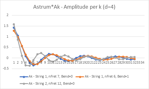
Note that the differences are much more significant between strings than they are between bend/no-bend on same string.
This shows that notes from different strings present themselves with a different signature (frequency and amplitudes). However, these signatures are also modified by many different parameters (time since strum, pickup placement, pickup height, action height, etc.), and are summed together with many shared harmonic frequencies. This makes it a difficult problem to solve with a traditional signal processing algorithm.
Equations
The previous sections described the general framework for the model of the sound recorded by a pickup, but did not show all the details, particularly how the scale compensation and bend amount impact all of the parameters. This section derives the equations more completely. The following diagram illustrates the geometry and variable symbols used in this section.
|
Name |
Symbol |
Units |
Range |
|
Scale Length (uncompensated) |
|
Inches |
24 to 27 |
Pickup Parameters per String:
|
Name |
Symbol |
Units |
Range |
|
Pickup Position (uncompensated) |
|
Inches |
0 (at bridge) to S (at nut) (Typical range: 0 to S/4) |
String Parameters:
|
Name |
Symbol |
Units |
Range |
|
Scale Compensation |
|
Inches |
|
|
Open Tuning Frequency |
|
Hz |
75 to 340 |
|
Damping Gamma |
|
None |
0.01 to 1.5 |
|
Radius |
|
inches |
0.003 to 0.030 (6 to 60 gauge) |
|
Linear Mass Density |
|
lb/in |
1x10⁻⁵ to 5x10e-4 |
|
Modulus of Elasticity |
|
lb*in/sec2 |
1x10¹⁰ to 1.2x10¹⁰ (185GPa to 215GPa) |
Strum Parameters:
|
Name |
Symbol |
Units |
Range |
|
Time since start of strum |
|
seconds |
0 to ~200 |
|
Force of Strum at t=t0 |
|
lb*in/sec2 |
0 to 4x10⁵ |
|
Strum Location along string at t=t0 (uncompensated) |
|
Inches |
0 (at bridge) to S (at nut) |
|
Fret Number |
|
Integer |
0 (open), 1-24 |
|
Bend, Number of Semitones |
|
Number |
0 to 5 (must be 0 for nFret=0) |
|
Phase (per harmonic) |
|
radian |
0 to 2π |
Transformed Variables:
|
Name |
Symbol |
Equation |
Units |
|
Fretted Position along string (uncompensated) |
|
|
Inches |
|
Longitudinal compression wave speed |
|
|
Inches/second |
|
|
|
|
Inches/second |
|
|
|
|
Inches/second |
|
|
|
Or
|
|
|
|
|
|
Inches/second |
|
Bend amount in number of half steps (semi-tones) |
|
|
Number |
|
Bend amount in distance |
|
|
Inches |
|
Fretted Position along bent string (compensated) |
|
Or
|
Inches |
|
Strum location |
|
Or
|
Inches |
|
Fundamental frequency |
|
|
Hz |
|
Modified Harmonic Index |
|
Where:
|
Number |
Primary Variables:
|
Name |
Symbol |
Equation, y(x,t) |
Equation, dy(x,t)/dt |
|
Strum Amplitude |
|
|
|
|
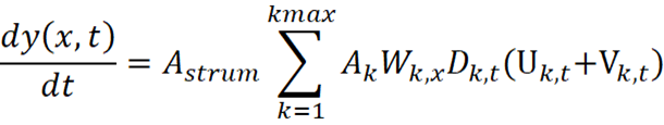
Harmonic Amplitude |
|
|
|
|
Standing Wave Shape |
|
|
|
|
Harmonic Damping |
|
|
|
|
String Vibration, sin |
|
|
|
|
String Vibration, cos |
|
|
|
Using the definitions for the primary variables in the table for y(x,t), the standing wave equation over time can be written as:
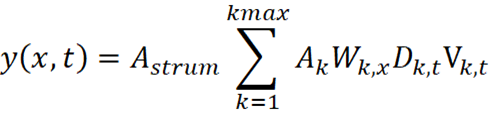
Using the definitions for the primary variables in the table for dy(x,t)/dt, the string vibration at a given x is modeled as:
For unplugged guitars, the vibration of the string (![]() ) at every x position induces
vibration of the guitar body (via the guitar soundboard and neck) which then
translates to a sound based upon the design of the guitar's size, material,
geometry, and construction.
) at every x position induces
vibration of the guitar body (via the guitar soundboard and neck) which then
translates to a sound based upon the design of the guitar's size, material,
geometry, and construction.
For electrified guitars, the pickup measures the string
vibration (![]() ) only at the x position of the
particular pickup (xpos). The output of multiple pickups at different x
positions are commonly combined together (via parallel or serial electronics)
and the combined signal is modified by the electronics and colored by the
amplifiers, producing the sound that is heard.
) only at the x position of the
particular pickup (xpos). The output of multiple pickups at different x
positions are commonly combined together (via parallel or serial electronics)
and the combined signal is modified by the electronics and colored by the
amplifiers, producing the sound that is heard.
Notes
Modulus of Elasticity Units
Note that units of the Modulus of Elasticity, E, is typically in either GPa (giga Pascals) or PSI (lb-force/in2). However, lb-force's unit is (lb*ft/s2) - thus the PSI numerator is relative to ft and the denominator is in terms of square inches, and lb-force is relative to gravity (32.174049 ft/s2) whereas pascals is not.
Thus, the conversion factors are as follows:
- {E in lb*in/sec2} = {E in psi:lb-force/in2} * 12*32.17
- {E in lb*in/sec2} = {E in GPa} * 1e9 * 2.20462/39.3701
Relationship between action height and scale compensation
From equations above, to keep the guitar intonated at a given fret, the bend necessary is calculated as:
![]()
Where:
![]()
The action height, b, can be calculated from the bend amount as follows:
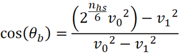
![]()
![]()